Building a Neural Network From Scratch

In this project we will learn what is an artificial neural network and how it can be used to train ML models.

To make this more practical, I will explain the theory based on a digit recognition project. You are more than welcomed to make changes to the code and see how it affects the model accuracy.

What are neural networks?

A typical neural network comprised of a node layers, containing an input layer, one or more hidden layers, and an output layer. Each node from one layer connects to all the nodes from another layer by weighted links. A weight is a measure of how significant a link is. In addition each node from the hidden and the output layers have a bias, while the weights can determine the slope of a function the bias allows the function to shift up and down. 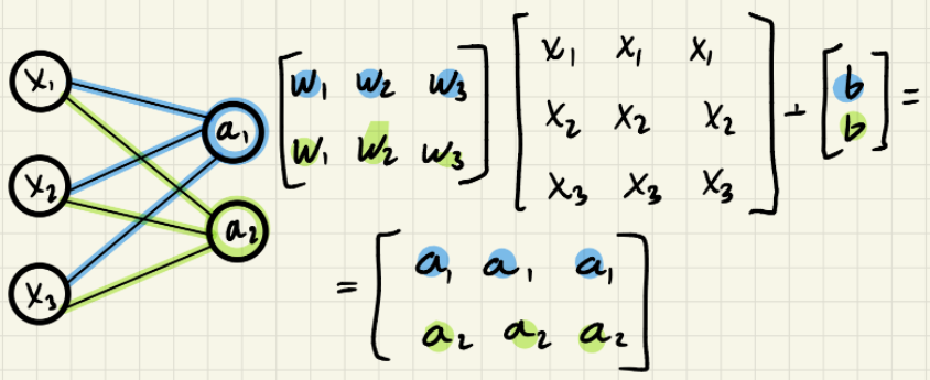We can refer to this as a linear function:

Designing a neural network to fit our needs

The data set we are going to use in this example consists of 42,000 training examples of handwritten digit images, each of size 28x28 pixels, where each pixel has a value between 0 and 255 representing the lightness and darkness of that pixel. In addition there is a label vector representing the true digit that was drawn.

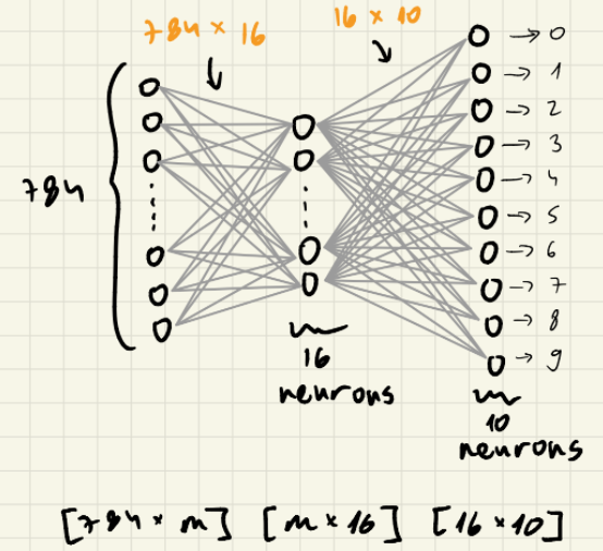
Our network will look like this:

• First layer: consists of 28x28 = 784 pixels
• Hidden layer: consists of (I chose 16 nodes) but it could be a different number.
• Output layer: consists of 10 nodes representing the digits 0-9.

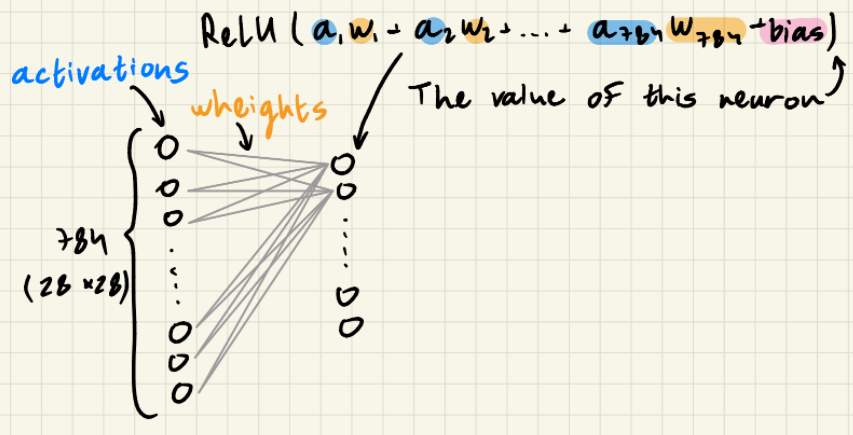
To get the activation value of the nodes in the next layer we need to perform the following calculation:

ReLU is an activation function, we will dive deeper into in the next section. We have 42,000 of this images, we are going to represent in a 784x42,000 matrix, each column is a representation of an image’s pixels values, we’ll call it X.
y is a vector of length 42,000 representing the labels.

The math behind

What are we looking for?

Implementation

Initializing the weight and biases matrices.
n is the size of the hidden layer.

def init_params(n):
    W1 = np.random.uniform(-0.5, 0.5, (n, 784))
    W2 = np.random.uniform(-0.5, 0.5, (10, n))
    b1 = np.zeros((n, 1))
    b2 = np.zeros((10, 1))
    return W1, b1, W2, b2

Determine the math functions described in the previous section.

# math functions
def ReLU(Z):
    return np.maximum(Z, 0)

def softmax(Z):
    A = np.exp(Z) / sum(np.exp(Z))
    return A

def ReLU_deriv(z):
    return (z > 0)*1

Here we make a matrix where each row is representing the digits and each representing the image’s label. Lets assume that the first image is 2, the first column will be [[0,0,1,0,0,0,0,0,0,0], […] ]

def one_hot_converter(y):
    one_hot = np.zeros((y.size, y.max() + 1))
    one_hot[np.arange(y.size), y] = 1
    return one_hot.T

Forward propagation - The neurons in the hidden layer receives input from all the neurons in the previous layer, combines it with its own set of weights and adds the bias. After applying some activation function (ReLU), calculates the output known as ‘hidden_activation’. The output of the hidden activation will serve as input for the next layer neurons. Similar calculations occur in the output layer except the fact that the activation function is the Softmax.

Backward propagation -

def forward_propogation(W1, b1, W2, b2, X):
    hidden_layer = W1.dot(X) + b1
    hidden_activation = ReLU(hidden_layer)
    output_layer = W2.dot(hidden_activation) + b2
    output_activation = softmax(output_layer)
    return hidden_layer, hidden_activation, output_layer , output_activation

def backward_propogation(hidden_layer, hidden_activation, output_layer , output_activation, W1, W2, X, y):
    one_hot = one_hot_converter(y)
    error_rate = output_activation - one_hot
    W2_deriv = 1 / m * error_rate.dot(hidden_activation.T)
    b2_deriv = 1 / m * np.sum(error_rate)
    hidden_layer_deriv = W2.T.dot(error_rate) * ReLU_deriv(hidden_layer)
    W1_deriv = 1 / m * hidden_layer_deriv.dot(X.T)
    b1_deriv = 1 / m * np.sum(hidden_layer_deriv)
    return W1_deriv, b1_deriv, W2_deriv, b2_deriv

def adjust_weights_and_biases(W1, b1, W2, b2, W1_deriv, b1_deriv, W2_deriv, b2_deriv, learning_rate):
    W1 = W1 - learning_rate * W1_deriv
    b1 = b1 - learning_rate * b1_deriv    
    W2 = W2 - learning_rate * W2_deriv  
    b2 = b2 - learning_rate * b2_deriv    
    return W1, b1, W2, b2

Applying a gradient descent algorithm to find the ‘minimal point’

def get_predictions(A2):
    return (A2).argmax(0)

def get_accuracy(predictions, Y):
    acc = np.sum(predictions == Y) / Y.size
    return acc

def gradient_descent(X, y, learning_rate, iterations):
    acc_list = []
    W1, b1, W2, b2 = init_params(16)
    for i in range(iterations):
        hidden_layer, hidden_activation, output_layer , output_activation = forward_propogation(W1, b1, W2, b2, X)
        W1_deriv, b1_deriv, W2_deriv, b2_deriv = backward_propogation(hidden_layer, hidden_activation, output_layer , output_activation, W1, W2, X, y)
        W1, b1, W2, b2 = adjust_weights_and_biases(W1, b1, W2, b2, W1_deriv, b1_deriv, W2_deriv, b2_deriv, learning_rate)
        if i % 10 == 0:
            print("Iteration No: ", i)
            predictions = get_predictions(output_activation)
            print(get_accuracy(predictions, y))
            acc_list.append(get_accuracy(predictions, y))
    print(acc_list)
    return W1, b1, W2, b2


W1, b1, W2, b2 = gradient_descent(X, y, 0.20, 350)

The results