Dementia Prediction

This article will deal with an attempt to build a model for predicting dementia as well as a brief description about this condition.

Dementia is a syndrome – usually of a chronic or progressive nature – in which there is deterioration in cognitive function (i.e. the ability to process thought) beyond what might be expected from normal ageing. It affects memory, thinking, orientation, comprehension, calculation, learning capacity, language, and judgement.
according to World Heath Organization: https://www.who.int/news-room/fact-sheets/detail/dementia

Treatment and care

There is no treatment currently available to cure dementia or to alter its progressive course. Numerous new treatments are being investigated in various stages of clinical trials. However, with early detection much can be offered to support and improve the lives of people with dementia, their carers, and families.

This post is all about data analysis, I will use the below data set in order to find some interesting insights about dementia syndrome.

Understanding The Data

The dataset I used is Cross-sectional MRI Data in Young, Middle Aged, Nondemented, and Demented Older Adults: This set consists of a cross-sectional collection of 416 subjects aged 18 to 96. For each subject, 3 or 4 individual T1-weighted MRI scans obtained in single scan sessions are included. The subjects are all right-handed and include both men and women. 100 of the included subjects over the age of 60 have been clinically diagnosed with very mild to moderate Alzheimer’s disease (AD). Additionally, a reliability data set is included containing 20 nondemented subjects imaged on a subsequent visit within 90 days of their initial session. Link to the dataset: https://www.kaggle.com/jboysen/mri-and-alzheimers

The attributes:

Subject ID - patient’s Identification
MRI ID - MRI Exam Identification
M/F - Gender
Hand - Dominant Hand
Age - Age in years
Group - Is the person Demented or Nondemented
Visit - Number of visits
Educ - Total years of education
SES - Socioeconomic status where 1 is the lowest status and 5 is the highest
MMSE - Mini Mental State Examination, in this test any score of 24 or more (out of 30) indicates a normal cognition. Below this, scores can indicate severe (≤9 points), moderate (10–18 points) or mild (19–23 points) cognitive impairment.
CDR - Clinical Dementia Rating. Ratings are assigned on a 0–5 point scale, (0 = absent; 0.5 = questionable; 1= present, but mild; 2 = moderate; 3 = severe; 4 = profound; 5 = terminal).
eTIV - Estimated Total Intracranial Volume (of the brain).
nWBV - Normalize Whole Brain Volume. Used to measure the progression of brain atrophy. expressed as decimal numbers between 0.64 to 0.89.
ASF - Atlas Scaling Factor is defined as the volume-scaling factor required to match each individual to the atlas target. Because atlas normalization equates to head size, the ASF should be proportional to eTIV.
MR Delay - unknown, no description had been provided. Since 99% of the column’s values are NA, we won’t use it.

Data Cleaning and Preprocessing

First of all we will load the data set and some useful Python packages, then we will clean the data.

import numpy as np
import pandas as pd
import matplotlib.pyplot as plt
import seaborn as sns

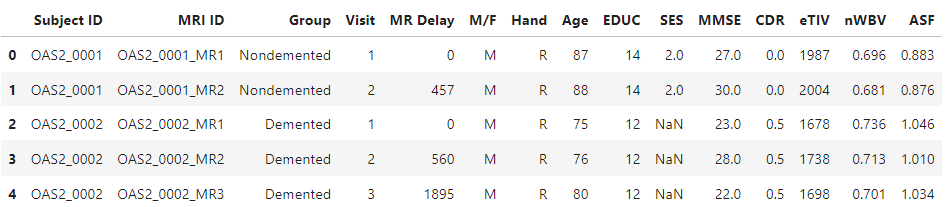
df = pd.read_csv('../input/mri-and-alzheimers/oasis_longitudinal.csv')
df.head()

  #We will change the values of the group column to 0 for Nondemented and 1 for Demented
  df.replace(to_replace='Nondemented', value=0, inplace=True, limit=None, regex=False, method='pad')
  df.replace(to_replace='Demented', value=1, inplace=True, limit=None, regex=False, method='pad')

  #Checking if there are a left handed patient
  df.Hand.unique()
  #Since this data set only right handed patients were examined so the #"hand" column does not contribute any valuable data for the prediction.
  df.drop(columns = ['Hand'])
  # Checking for null values
  df.isnull().sum()

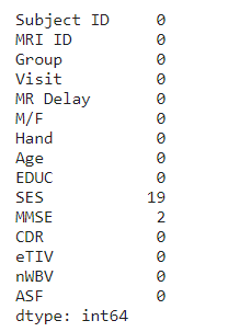
We can now see that SES and MMSE columns have 19 and 2 null values respectively. Remember that SES value stands for ‘Socioeconomic status’, since our data contains 373 entries, dropping out 19-21 rows would mean loosing ~5% of data. Another reason to not drop those rows is that people with low socioeconomic status are more likely to hide this information, the resulting collection of data would have a series of missing values. To prevent our data becoming smaller and more biased we’ll use the mean of the SES score to fill out the nulls.

mean_value = df['SES'].mean()

# Replace nulls in column SES with the mean of values in the same column
df['SES'].fillna(value=mean_value, inplace=True)
df.isnull().sum()

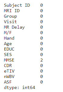
#drop the remaining 2 rows containing null values
df.dropna()

Data Visualization

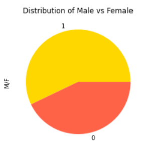
# male=0 & female=1
df['M/F'].value_counts().plot(kind='pie', colors = ['gold','tomato'],
title = 'Distribution of Male vs Female'))

#where 0 =nondimented, 1 =dimented
df['Group'].value_counts().plot(kind='pie',colors=['orange','dodgerblue','blue'],
title = 'Distribution of Dimented vs Nondimented')

fig = plt.figure(figsize=(10,8))
sns.catplot(x='CDR',y='Age',data=df,hue='M/F', palette='hls')

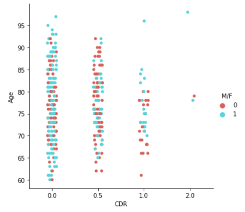
fig = plt.figure(figsize=(10,8))
sns.catplot(x='CDR',y='Age',data=df,hue='Group', palette='hls')

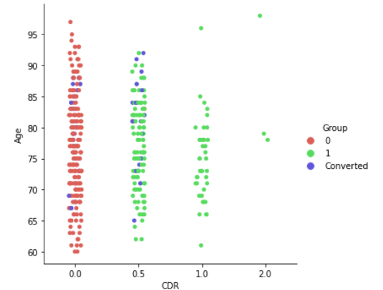
fig = plt.figure(figsize=(10,8))
sns.catplot(x='CDR',y='EDUC',data=df,hue='CDR', palette='hls')

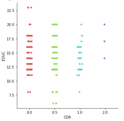
fig = plt.figure(figsize=(10,8))
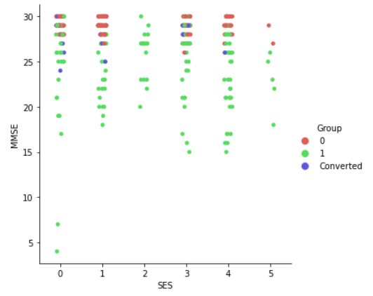
sns.catplot(x='SES',y='MMSE',data=df, hue='Group', palette='hls')

fig, ax =plt.subplots(1,2,figsize=(10,6))
sns.stripplot(x='CDR',y='ASF',data=df,ax=ax[0], palette='hls')
sns.stripplot(x='CDR', y='nWBV', data=df,ax=ax[1], palette='hls')

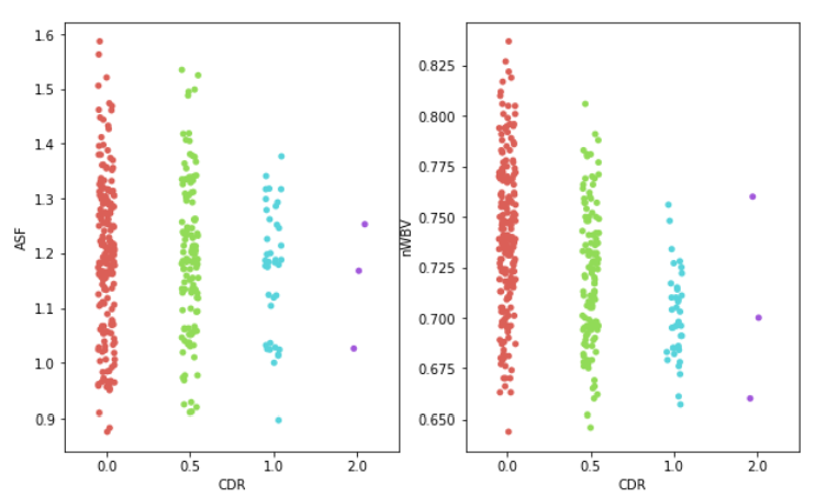
fig = plt.figure(figsize=(10,8))
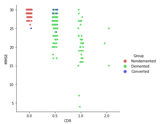
sns.catplot(x='CDR',y='MMSE',data=df, hue='Group', palette='hls')

plt.figure(figsize=(14, 8))
sns.heatmap(df.corr(), annot=True)
plt.show()

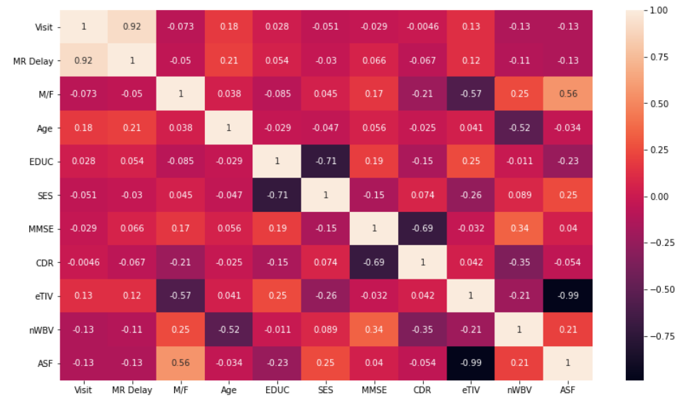
Since eTIV and ASF have very strong negative correlation (-0.99), we’ll drop one of those columns.

Model creation

Here comes the interesting part! First we will define the target column and split the dataframe into train and test sets:

y = df.loc[:, ['Group']]
X = df.iloc[:, 3:]
X_train,X_test,y_train,y_test = train_test_split(X,y,random_state=1)

Building the decision tree model

We will conduct cross-validation in order to set the hyper-parameters so that it will increase the performance of the resulting tree as much as possible.

from sklearn.tree import DecisionTreeClassifier
from sklearn.model_selection import cross_val_score
from sklearn.metrics import confusion_matrix, accuracy_score, recall_score, roc_curve, auc
best_score = 0
for dep in range(1, 12): # there are 11 different features
    clf = DecisionTreeClassifier(random_state=1, max_depth=dep, criterion='gini')
    scores = cross_val_score(clf, X_train, y_train, cv=4, scoring='accuracy')
        # compute mean cross-validation accuracy
    score = np.mean(scores)

    # if we got a better score, store the score and parameters
    if score > best_score:
        best_score = score
        best_depth = dep

# Rebuild a model on the combined training and validation set        
selected_model = DecisionTreeClassifier(max_depth=best_depth).fit(X_train, y_train)

test_score = selected_model.score(X_test, y_test)
pred_output = selected_model.predict(X_test)
test_recall = recall_score(y_test, pred_output, pos_label=1, average='weighted')
#fpr - false positive rate, tpr - true positive rate
fpr, tpr, thresholds = roc_curve(y_test, pred_output, pos_label=1)
test_auc = auc(fpr, tpr)
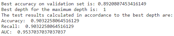
print("Best accuracy on validation set is:", best_score)
print("Best depth for the maximum depth is: ", best_depth)
print("The test results calculated in accordance to the best depth are:")
print("Accuracy: ", test_score)
print("Recall: ", test_recall)
print("AUC: ", test_auc)

Plotting the decision treatment

from sklearn.tree import export_graphviz
import graphviz
dot_data=export_graphviz(selected_model, feature_names=X_train.columns.values.tolist(),out_file=None)
graph = graphviz.Source(dot_data)  
graph

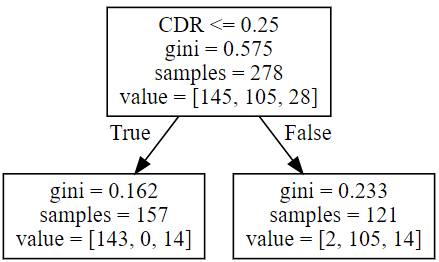
Conclusions

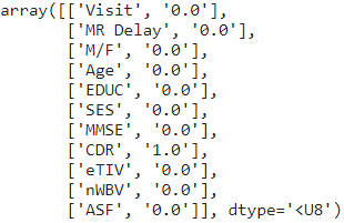
As we can see from the graph above the most important feature is the CDR, by printing the feature importance we see that this feature is the only one that was taken into account when the tree was built.

 np.array([X.columns.values.tolist(), list(selected_model.feature_importances_)]).T